A Sharpe Approach to Position Sizing

As we look back at the Paris Olympics and European Football Championship (albeit somewhat painfully as an Englishman), we are reminded that teamwork is key to success. Games are not won by fielding your strongest player in isolation; strengths need to be matched across teammates, time and energy on the pitch or court applied judiciously, and poor patches managed with precision.

‍

This holds for investment portfolios as it does in sports. Last month, Cameron Hight looked at how an investment manager might assess volatility and downside risk for discrete outcomes. Such binomial outcomes - either A or B happens with known frequencies and payoffs - are frequently found in the world of gambling, but less so in finance.

‍

Stocks form continuous distributions (not binomial) where volatility informs us about the likelihood of return at different levels. While Kelly sizing can be adapted to apply to portfolios of risk assets, the associated rebalancing costs and implied leverage tend to preclude it from consideration. Not for nothing, Kelly sizing is often referred to as "the boundary where allocation goes from aggressive to insane."

‍

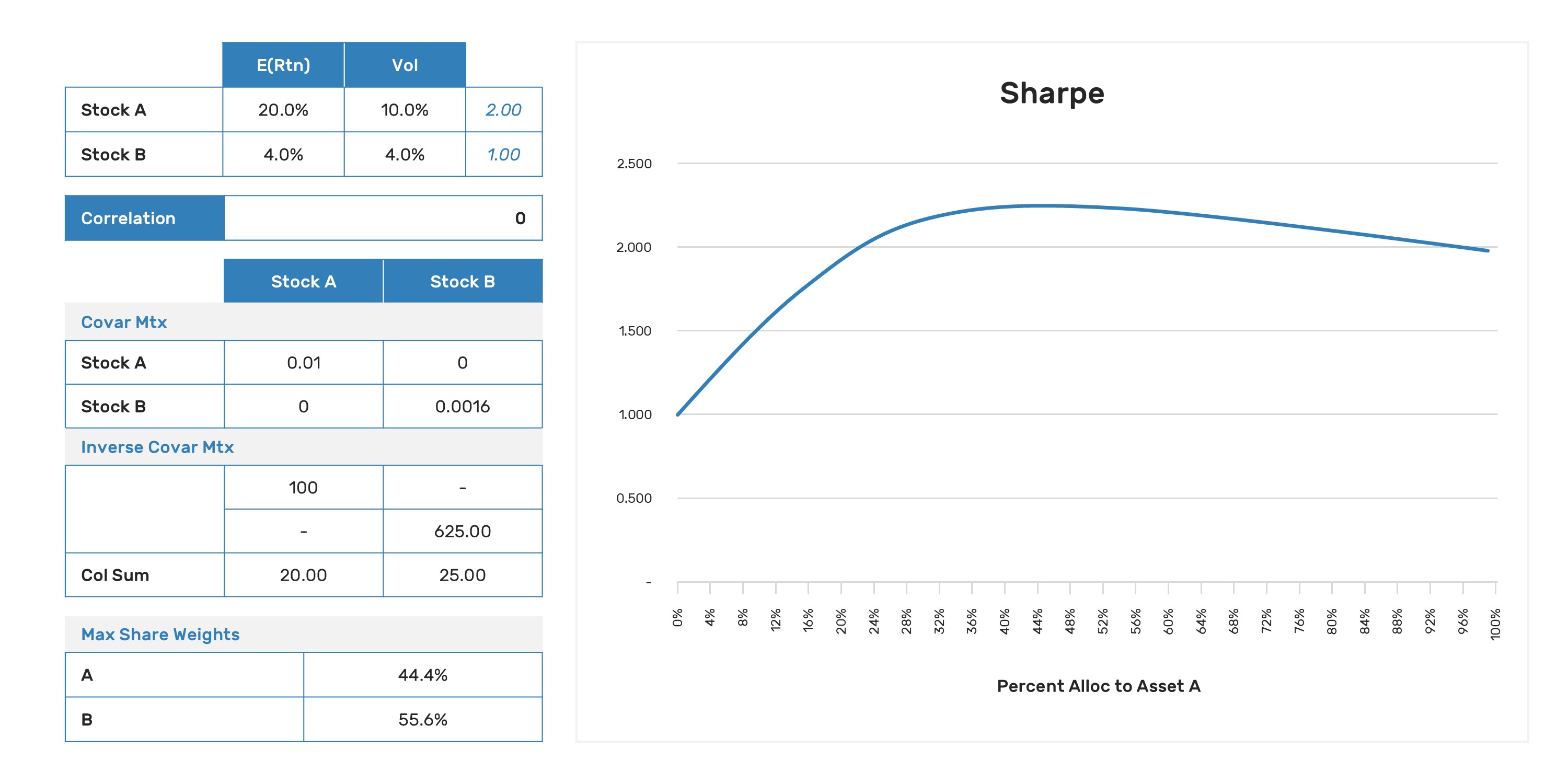
Imagine we have two positions in our portfolio with estimates of the forward Sharpe ratio for each. We'll assume for the moment that the risk-free rate is zero and that the two assets are uncorrelated. Position A has an estimated Sharpe of 2.0, and position B has an estimated Sharpe of 1.0. How should we optimally allocate our capital to those positions in order to maximize the estimated Sharpe of the combined portfolio? Generally, people's guesses to this question will range from "proportional to the Sharpes" through "all of it in the Sharpe 2 position," up to the too-cool-for-school "proportional to the square of the Sharpes."

‍

The reality is that it depends. More precisely, it depends on the volatility of the underlying assets. "But isn't that already part of the Sharpe?". It is, but that is only part of the story. For uncorrelated positions, the optimal Sharpe-maximizing allocation is to size proportionally to Sharpe, which is further divided by volatility(1). We can prove that with math, or we can look at a simple example:

‍

Zero Correlation Example

Mathematically, this means that if you have two assets, A and B, with Sharpe ratios 𝑆𝐴SA​ and 𝑆𝐵SB, and volatilities 𝜎𝐴σA and 𝜎𝐵σB, the optimal allocation weights​ are:

‍

‍

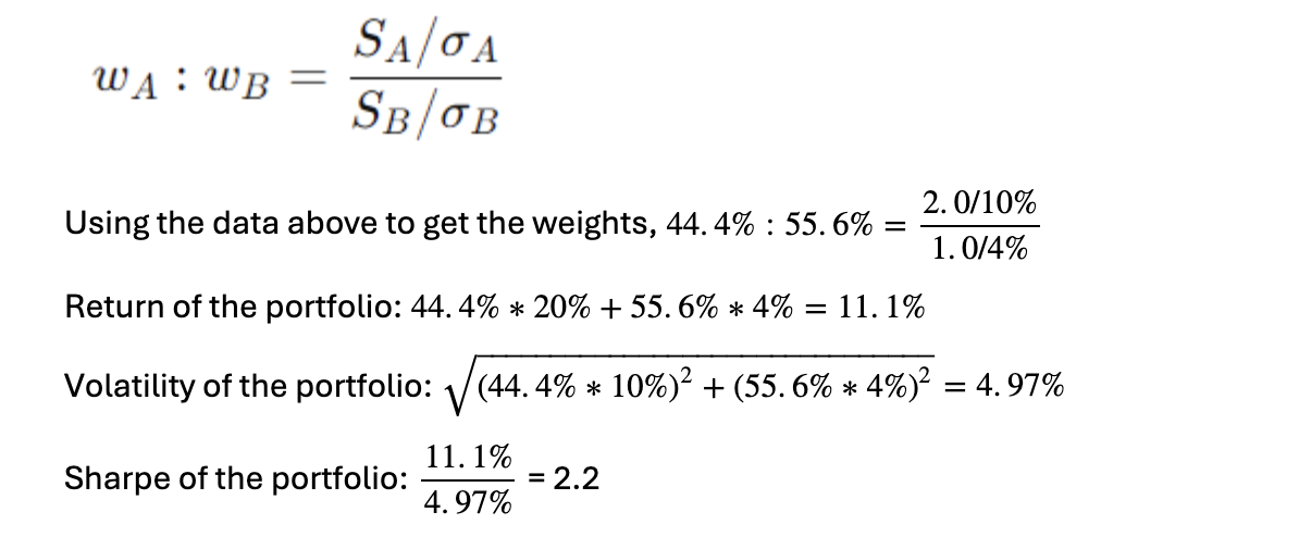
Here we see that Stock B with a lower Sharpe of 1.0 ends up with a greater weighting than Stock A which has a 2.0 Sharpe and the combination results in a still higher overall Sharpe of 2.2.

‍

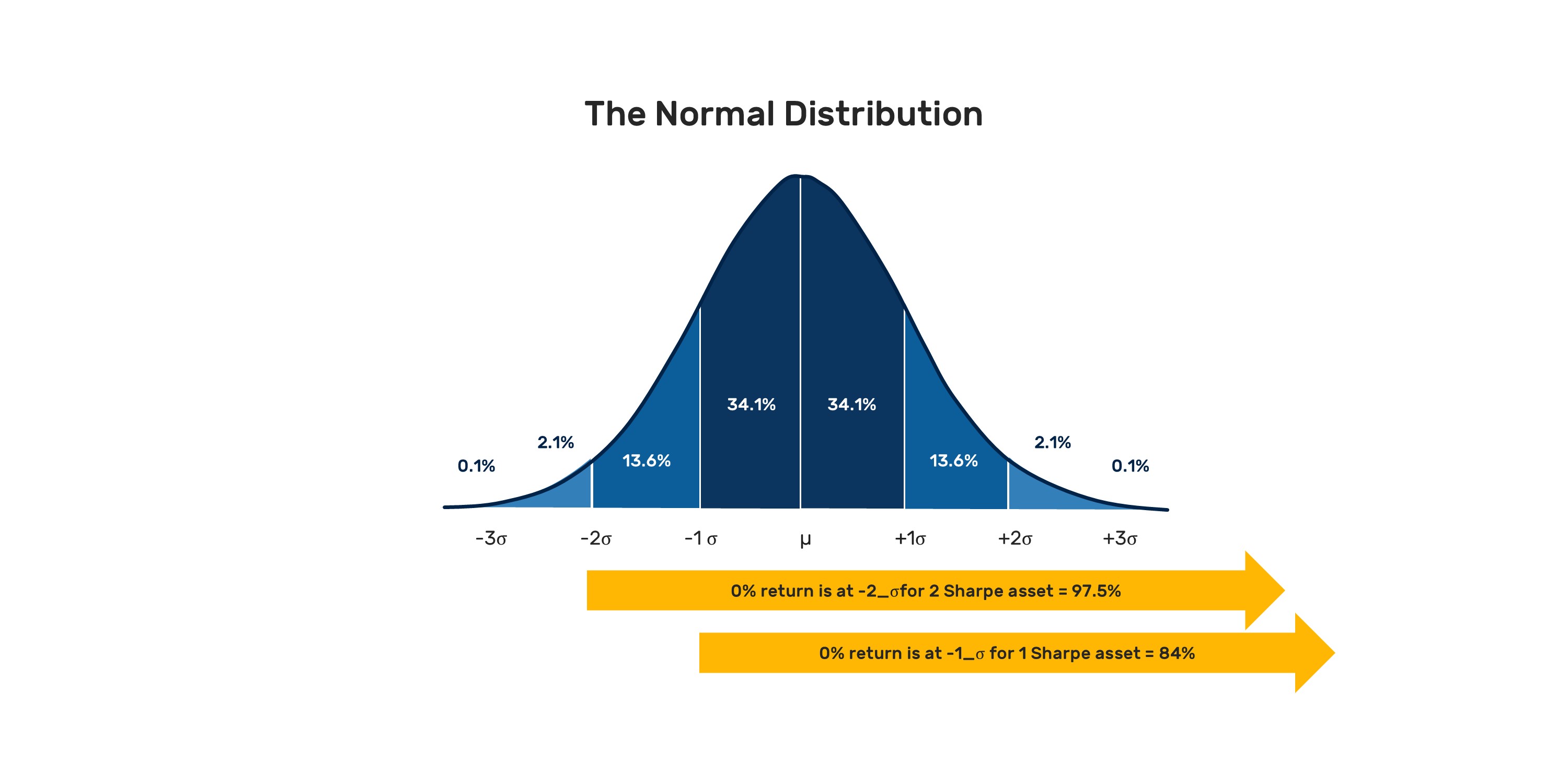
We can think about this result in a strict mathematical sense(2), or we can think about the intuition behind what Sharpe and volatility mean. Sharpe is one way to understand our "edge" in a trade; while we cannot predict the future perfectly, an estimate of our Sharpe provides a framework for thinking about the likelihood of coming out ahead.

‍

Our Sharpe 1.0 position should have positive returns 84% of the time, while our Sharpe 2.0 position should have positive returns 97.5% of the time(3). The problem we face is that we need to manage the distribution of this edge, which is where volatility comes in.

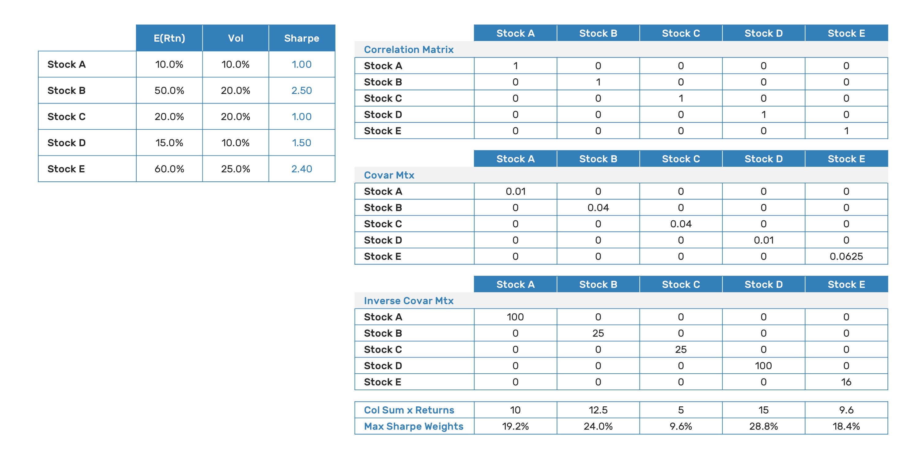
Correlated Example

Of course, the portfolios we build are never composed of uncorrelated assets(4). The framework still works; however, the optimal weighting for our assets is proportional to the inner product of the inverted covariance matrix columns and the expected returns. With a little algebra, this can be seen to be directly analogous to the uncorrelated example above (and tested by setting the correlations of the assets to zero to observe the same outcome):

Given the simplicity of the optimal weighting of capital to maximize Sharpe, why is portfolio construction so difficult? The answer lies in the underlying assumptions we have made:

‍

1. Expected returns are known in advance. This is rarely the case, although Alpha Theory provides portfolio managers with the ability to think strategically and more accurately about expected returns, leading to better-calibrated inputs.
   ‍
2. Volatility and covariance are known in advance. While this, too, requires a supernatural degree of foresight, the ability of modern multi-factor risk models to capture the key salient driver of volatility and attach well-calibrated estimates to both volatility and covariance is impressive and alleviates a material degree of concern. Conversely, if you use individual asset historic price return data, the outcome will materially lack robustness.
   ‍
3. The portfolio is free from constraints. This is, again, rarely the case. Portfolio managers must juggle multiple and often conflicting demands on the end portfolio. As we move from the theoretical to the practical, a modern optimizer is the preferred approach to finding efficient solutions, at least in the Pareto sense of the word.
   ‍

Hopefully, this post and its predecessor have given you some insight into why volatility management is at least as important as return estimation when it comes to portfolio construction. Alpha Theory offers portfolio managers insights into both, while our work at CenterBook Partners involves taking these concepts to their ultimate evolution, helping managers extract and monetize crucial idiosyncratic returns from their investment research and portfolios.

‍

‍

(1) Alternatively, as Sharpe is return divided by volatility and variance is the square of volatility, the Sharpe maximizing allocation is return divided by variance. We'll see this applied again below.

(2) Quant Exchange

(3) Sobering statistics and worth bearing in mind next time you hear of a manager with a proclaimed Sharpe of 2.0; the inference being that they underperform cash once every 40 years. Of course, this is all predicated on an assumption of normally distributed returns.

(4) Although at CenterBook, we hedge out correlated risk assiduously and that leaves us with a portfolio where the key driver of risk is the uncorrelated idiosyncratic component of the individual assets.

‍

About the Author:

Chris White has over two decades of experience in hedge fund asset management, specializing in quantitative investment, alpha capture, and risk management. Prior to joining CenterBook Partners, Chris was Head of Alpha Strategies and Co-Head of Quant for Graticule Asset Management Asia, where he ran internal alpha capture and built the firm’s center book. He was formerly a partner of Nezu Asia Capital Management, where, as Head of Portfolio Construction and Risk, he was responsible for the systematic implementation of fundamental alpha sources. Before joining the Nezu Group, Chris was Portfolio Manager and Director of Risk and Quantitative Strategies at Elmwood Advisors, where he ran market-neutral quantitative equity strategies. Previously, Chris served as Senior Vice President and Head of Equity Risk at Financial Risk Management (FRM) in Tokyo and New York. Chris had also served as Manager of Quantitative Equity Sales and Research at Schroder Securities Japan. He began his career working for Cazenove Securities in London and Tokyo in Equity Sales and Research. Chris graduated with an L.L.B. in English Law & Japanese Language from Cardiff University (UK)/Obirin University (Tokyo).

‍

This blog post (the “Blog”) does not describe or seek to offer any advisory services and is not an “advertisement”, as defined in SEC Rule 206(4)-1. Accordingly, nothing in this Blog should be considered investment advice, nor establishes an advisory relationship. The summary description of the sharpe approach to position sizing included herein is intended only for informational purposes and are not intended to be complete. The Presentation is not intended as an offer or solicitation with respect to the purchase or sale of any security.